Análise Fatorial Exploratória - EFA

library(tidyverse) 
library(janitor)
library(gt)
library(PerformanceAnalytics)
library(plotly)
library(kableExtra)
library(ggrepel)
library(factoextra)
library(psych)

Base de Dados

# Selecionar variáveis quantitativas
df <- mtcars |> 
select (mpg, disp, hp, drat, wt, qsec) |> 
data.frame()

df_std <- scale(df) |> data.frame()

Correlações

chart.Correlation(df, histogram = TRUE, method = "pearson")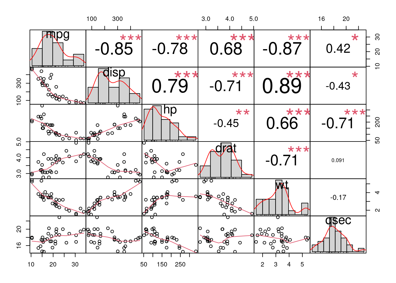

DataExplorer::plot_correlation(df)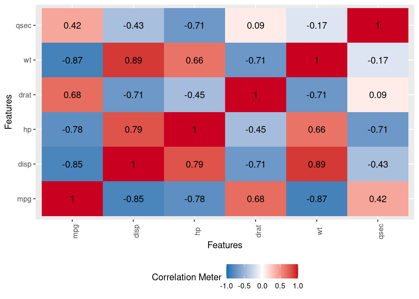

#outra opcão:

corrplot::corrplot(cor(df, use="complete.obs"), order = "hclust", tl.col='black', tl.cex=.75, addCoef.col = T)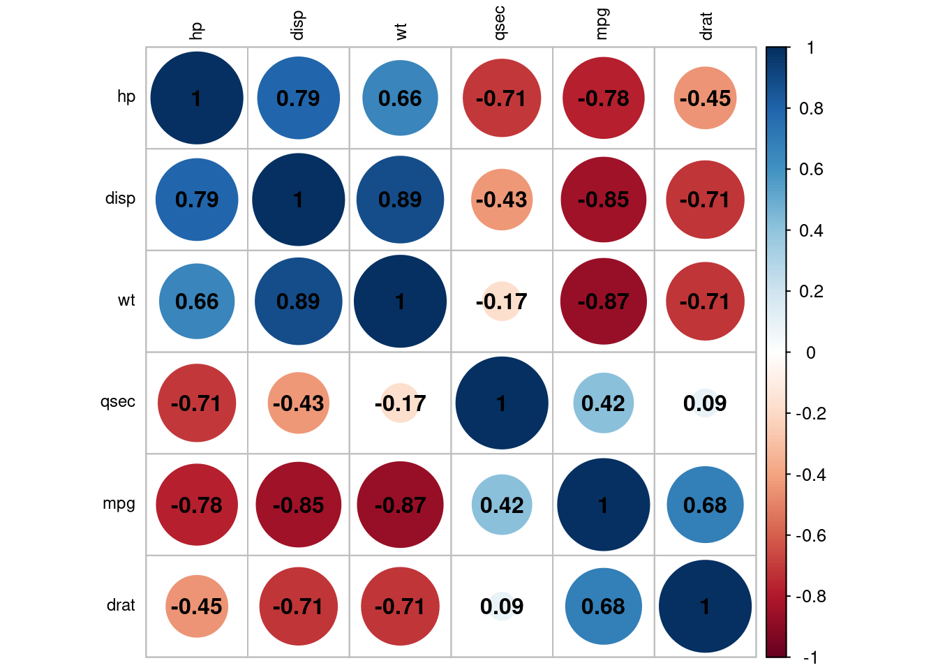 

KMO e Bartlett

Verificamos se os dados estão adequados para uma análise fatorial.

KMO

#Cutoff sugerido (Kairse 1974) >= 60.
psych::KMO (r = cor(df))

Kaiser-Meyer-Olkin factor adequacy
Call: psych::KMO(r = cor(df))
Overall MSA =  0.76
MSA for each item = 
 mpg disp   hp drat   wt qsec 
0.83 0.78 0.83 0.85 0.70 0.52 

Teste de esfericidade de Bartlett

Validar homogeneidade da variância

bartlett.test(df)

    Bartlett test of homogeneity of variances

data:  df
Bartlett's K-squared = 831.17, df = 5, p-value < 2.2e-16

EFA

Análise Fatorial Exploratória

Nossos dados passaram com nível de significância de 5%.

#EFA Sem rotação, com maxima verossemelhanca (ML).

efa <- factanal(~ ., data= df_std, factors = 3, rotation = "none")
efa

Call:
factanal(x = ~., factors = 3, data = df_std, rotation = "none")

Uniquenesses:
  mpg  disp    hp  drat    wt  qsec 
0.005 0.005 0.183 0.406 0.095 0.005 

Loadings:
     Factor1 Factor2 Factor3
mpg  -0.922  -0.266   0.272 
disp  0.928   0.247   0.271 
hp    0.890  -0.155         
drat -0.629  -0.441         
wt    0.812   0.493         
qsec -0.666   0.742         

               Factor1 Factor2 Factor3
SS loadings      4.003   1.145   0.153
Proportion Var   0.667   0.191   0.026
Cumulative Var   0.667   0.858   0.884

The degrees of freedom for the model is 0 and the fit was 0.0414 

# SS Loadings: Estes são as somas dos quadrados (SS) das cargas, ou seja, os eigen values.
# .Eles explicam as variancias de todas as variáveis de determinado fator.

# Como regra geral (Kaiser), se um fator tem eigenvalue maior que 1, ele é importante.
# Neste caso, fatores 1 e 2 parecem ser importantes. Este valor pode ser calculado a partir das cargas: Ex: sum(efa$loadings[,1]^2) para o ev do primeiro fator.]

#A comunalidade, é a soma dos quadrados de todos os fatores dada uma vaiável. A Singularidade é 1- Comunilidade. Por exemplo. Para a variável mpg temos Uniqueness = (1- sum(efa$loadings[1,]^2))

cargas <- efa$loadings[,1:3]
plot(cargas, type = "n")
text (cargas, labels = names(df), cex=.7)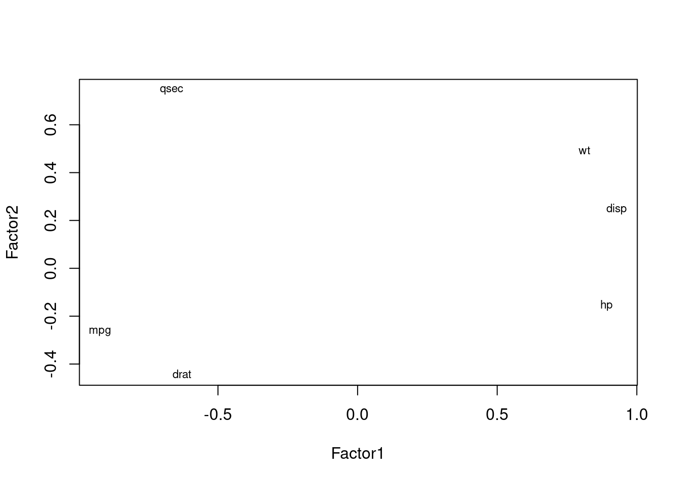

data.frame(cargas) |>
  mutate(var = names(df)) |> 
  pivot_longer(cols = !var) |> 
  mutate(var = factor(var)) |>
  ggplot(aes(x = var, y = value, fill = var)) +
  geom_col() +
  facet_wrap(~name) +
  labs(x = NULL, y = NULL, fill = "Legenda:")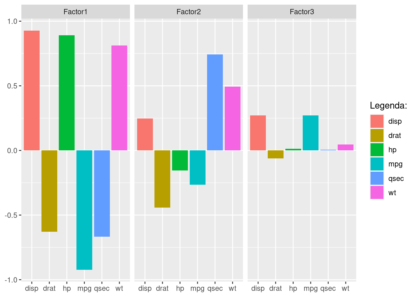 

Rotacionando a matriz

# Usando varimax
efa_rot <- factanal(~ ., data= df_std, factors = 3, rotation = "varimax")
efa_rot

Call:
factanal(x = ~., factors = 3, data = df_std, rotation = "varimax")

Uniquenesses:
  mpg  disp    hp  drat    wt  qsec 
0.005 0.005 0.183 0.406 0.095 0.005 

Loadings:
     Factor1 Factor2 Factor3
mpg  -0.825   0.361   0.428 
disp  0.911  -0.391   0.107 
hp    0.590  -0.676  -0.105 
drat -0.766                 
wt    0.936  -0.122  -0.119 
qsec          0.995         

               Factor1 Factor2 Factor3
SS loadings      3.326   1.749   0.226
Proportion Var   0.554   0.291   0.038
Cumulative Var   0.554   0.846   0.884

The degrees of freedom for the model is 0 and the fit was 0.0414 

cargas <- efa_rot$loadings[,1:3]
plot(cargas, type = "n")
text (cargas, labels = names(df), cex=.7)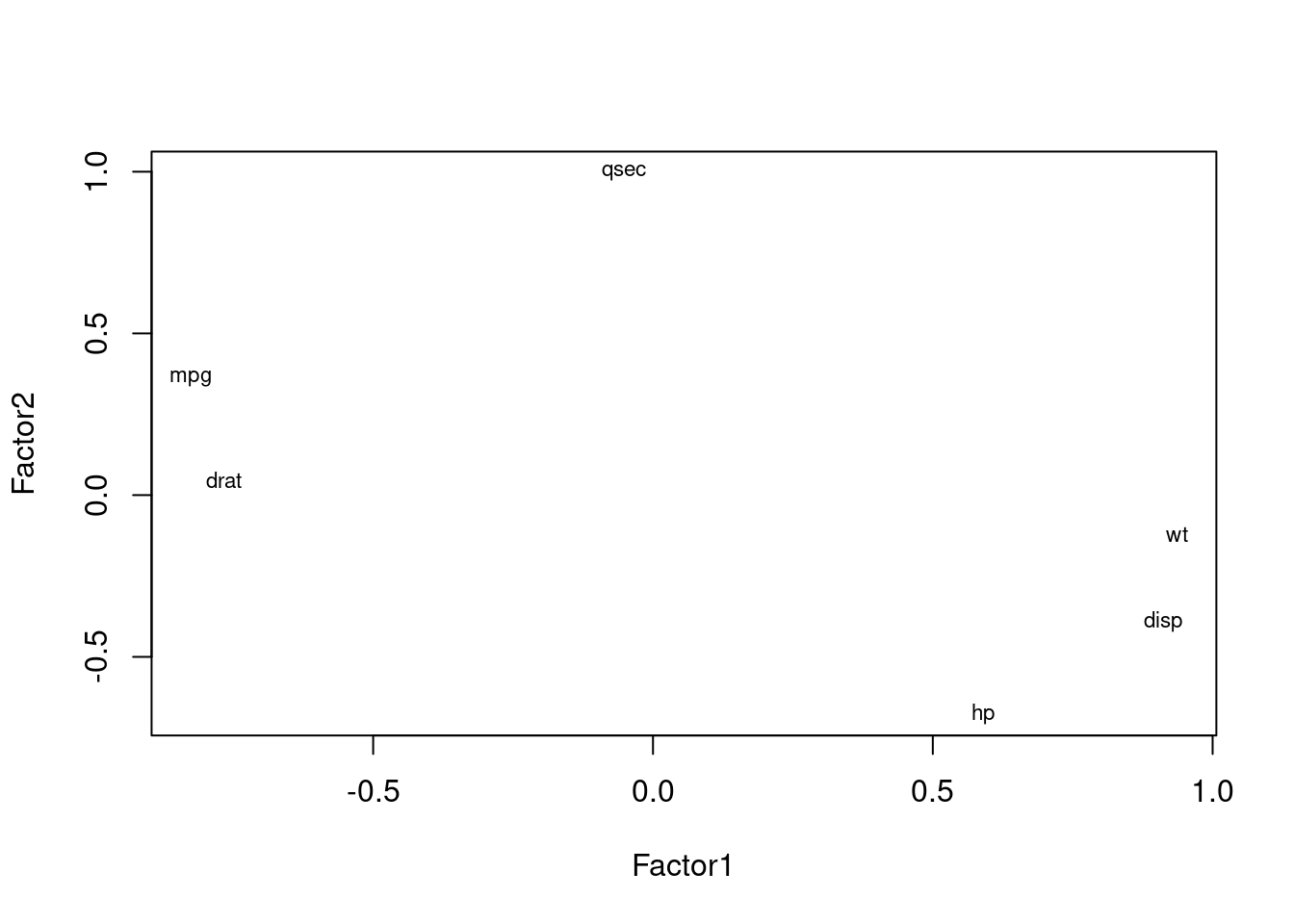

data.frame(cargas) |>
  mutate(var = names(df)) |> 
  pivot_longer(cols = !var) |> 
  mutate(var = factor(var)) |>
  ggplot(aes(x = var, y = value, fill = var)) +
  geom_col() +
  facet_wrap(~name) +
  labs(x = NULL, y = NULL, fill = "Legenda:")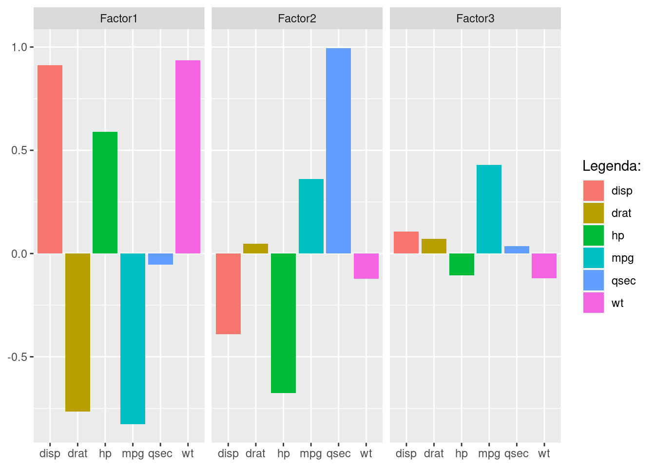 

Análise Paralela

corpdat1 <- cor(df, use="pairwise.complete.obs")
fa.parallel(x=corpdat1, fm="minres", fa="fa")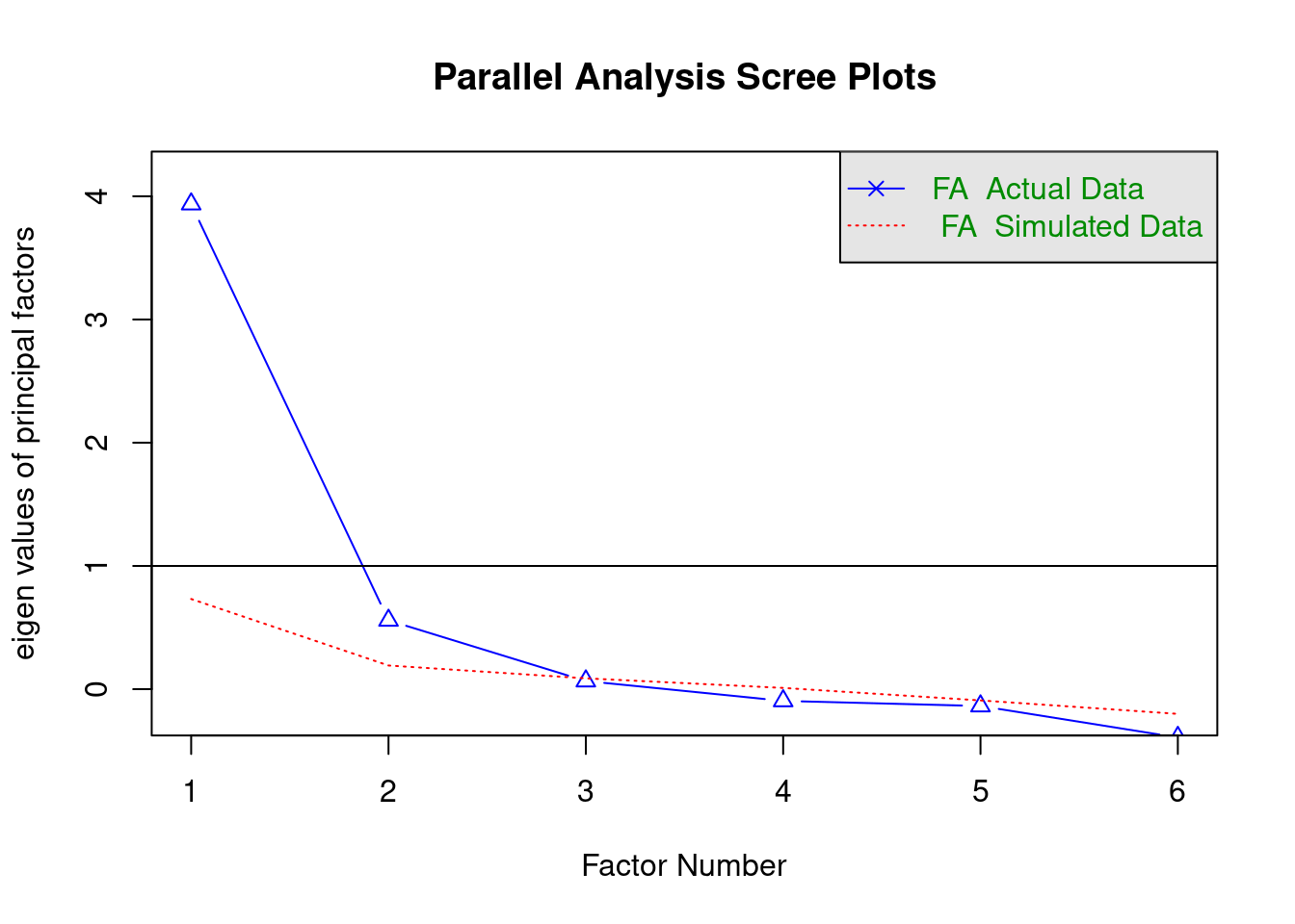

Parallel analysis suggests that the number of factors =  2  and the number of components =  NA