Base de Dados

# Selecionar variáveis quantitativas
df <- mtcars |> 
select (mpg, disp, hp, drat, wt, qsec) |> 

# Fazer o z-score (padronizacao)  
scale() |> data.frame()

Correlações

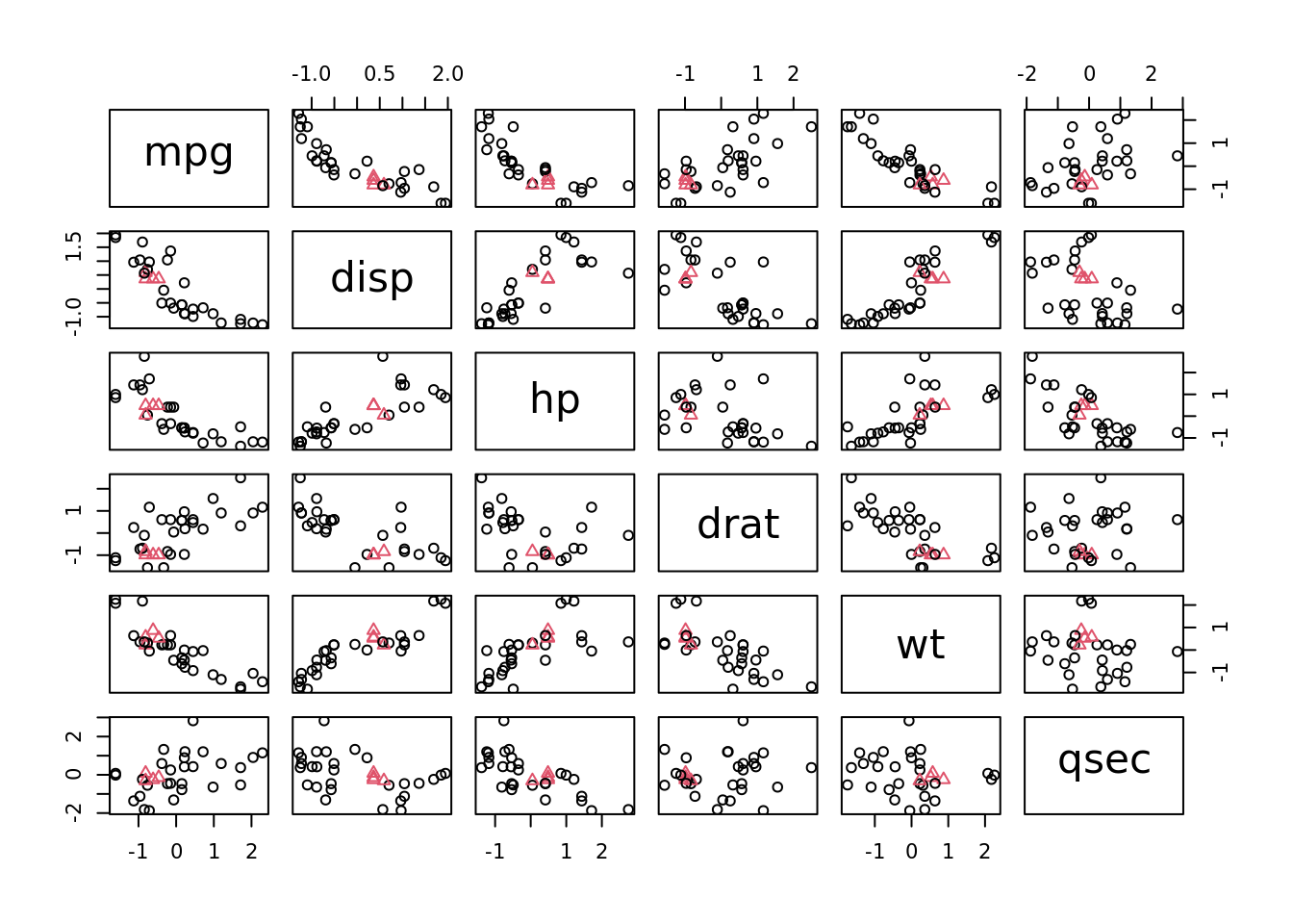
chart.Correlation(df, histogram = TRUE, method = "pearson")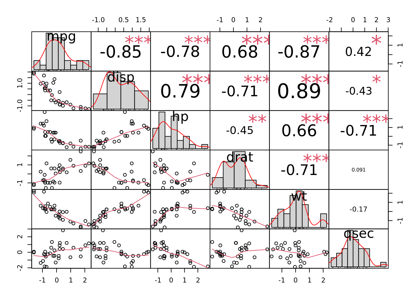

DataExplorer::plot_correlation(df)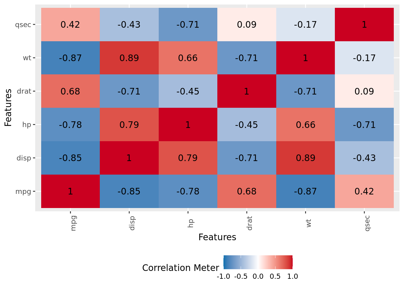

Método Hierárquico

Usando hclust

#calcular as distancias da matriz utilizando a distancia euclidiana
distancia <- dist(df, method = "euclidean")

#Calcular o Cluster
clusterh <- hclust(distancia, method = "single" )

# Dendrograma
plot(clusterh, cex = 0.6, hang = -1)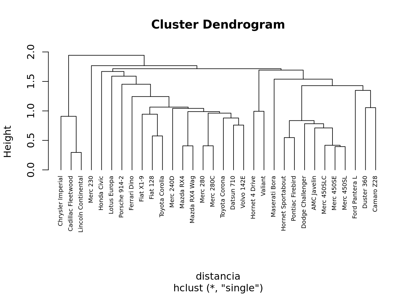

#Metodo Elbow
fviz_nbclust(df, FUN = hcut, method = "wss")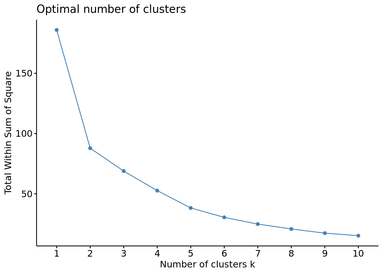

#criando 5 grupos
clusterh_grupos <- cutree(clusterh, k = 5)
table(clusterh_grupos)

clusterh_grupos
 1  2  3  4  5 
15  2 11  1  3

#transformando em data frame a saida do cluster
grupo_hierarquico <- data.frame(clusterh_grupos) |> 
  dplyr::rename (cluster = last_col())

df_final <- bind_cols(mtcars, grupo_hierarquico)

df_final_EDA <- df_final |>  pivot_longer(cols = c(1,3:7))

plot_final_EDA <- df_final_EDA |> 
  ggplot(aes(x=cluster, y=value, color= as_factor(cluster)))+
  #geom_jitter(alpha = 0.5, size = 6, width = 0.1)+
  geom_boxplot()+
  facet_grid(scales = "free_x", cols = vars(name))

plot_final_EDA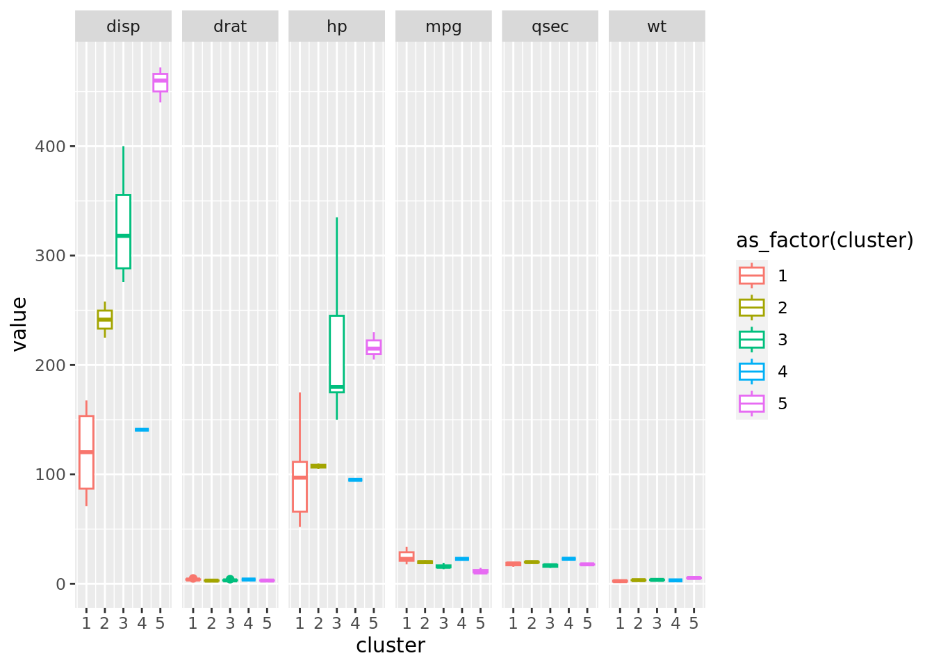

Usando agnes

#Comparar os tipos de link
m <- c( "average", "single", "complete", "ward")
names(m) <- c( "average", "single", "complete", "ward")

map(m, ~agnes(df, method = .)$ac)

$average
[1] 0.7659485

$single
[1] 0.5631059

$complete
[1] 0.867514

$ward
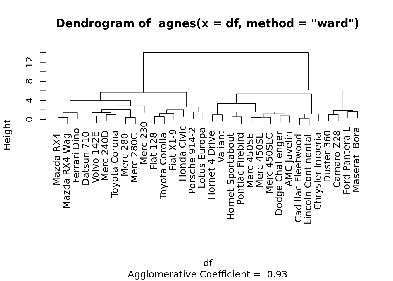
[1] 0.9320082

#Calcular o Cluster
clustera <- agnes(df, method = "ward" )

# Dendrograma
pltree(clustera, cex = 0.6, hang = -1)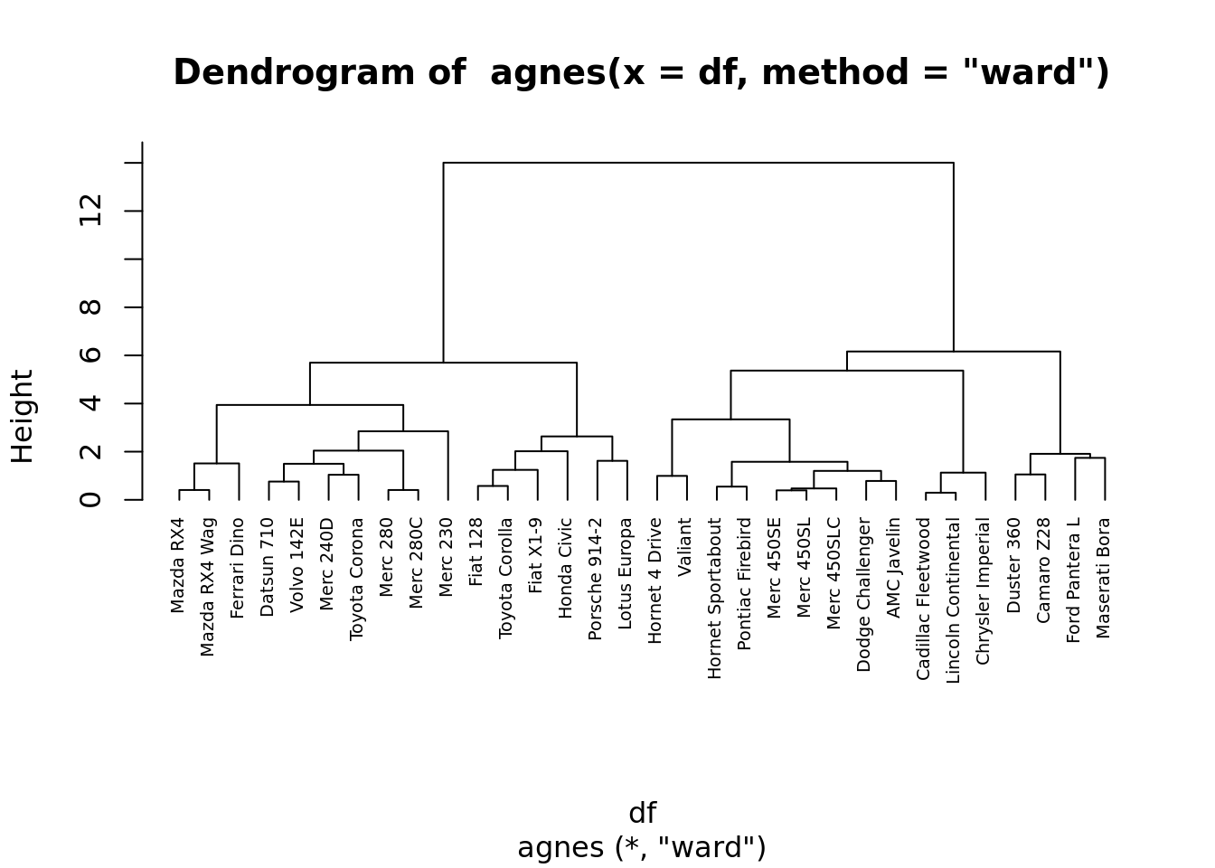

#Agnes plot ( dendograma e banner plot)
plot(clustera)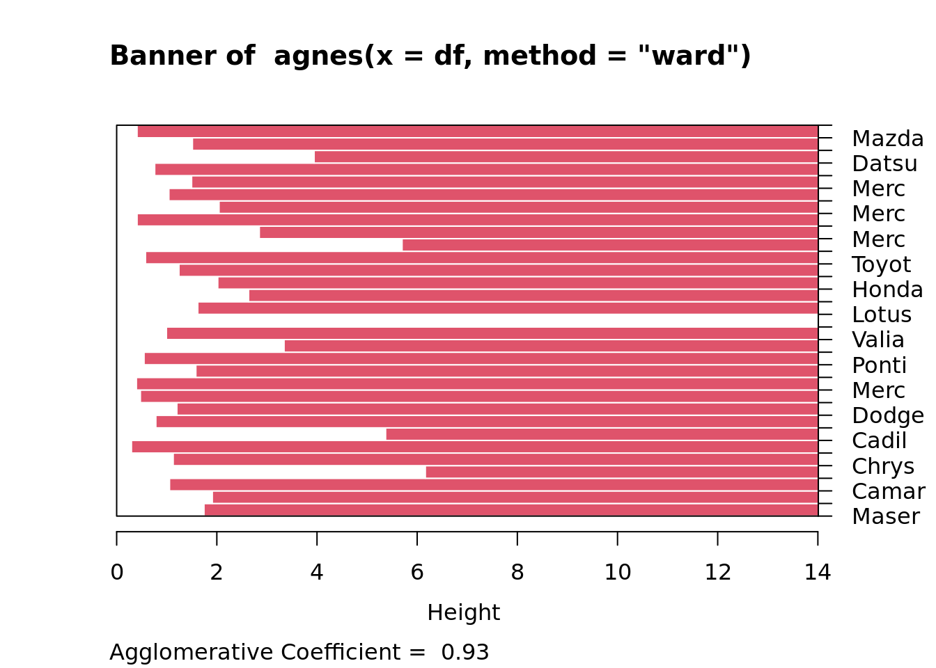

#criando 5 grupos
clustera_grupos <- cutree(clustera, k = 5)
table(clustera_grupos)

clustera_grupos
 1  2  3  4  5 
10  9  4  3  6

#transformando em data frame a saida do cluster
grupo_hierarquico_a <- data.frame(clustera_grupos) |> 
  dplyr::rename (cluster = last_col())

df_final <- bind_cols(mtcars, grupo_hierarquico)

df_final_EDA <- df_final |>  pivot_longer(cols = c(1,3:7))

plot_final_EDA <- df_final_EDA |> 
  ggplot(aes(x=cluster, y=value, color= as_factor(cluster)))+
  #geom_jitter(alpha = 0.5, size = 6, width = 0.1)+
  geom_boxplot()+
  facet_grid(scales = "free_x", cols = vars(name))

plot_final_EDA

Warning

Veja que agnes(*, method=“ward”) corresponde a hclust(*, “ward.D2”).

Método Não-Hierárquico

K-Means

O número de cluster (k) precisa ser dado

#Método Elbow
fviz_nbclust(df, FUN = hcut, method = "wss")

#Gerando clsuters com 3, 4, 5 e 6 grupos
k3 <- kmeans(df, centers = 3)
k4 <- kmeans(df, centers = 4)
k5 <- kmeans(df, centers = 5)
k6 <- kmeans(df, centers = 6)

lista <- list(k3,k4,k5,k6)
names(lista) <- c("k3", "k4", "k5", "k6")

G <- map(lista, ~fviz_cluster(., geom = "point", data = df) +
           ggtitle(paste(length(
             (pluck(., 7))),"clusters")))

G$k3 + G$k4 + G$k5 + G$k6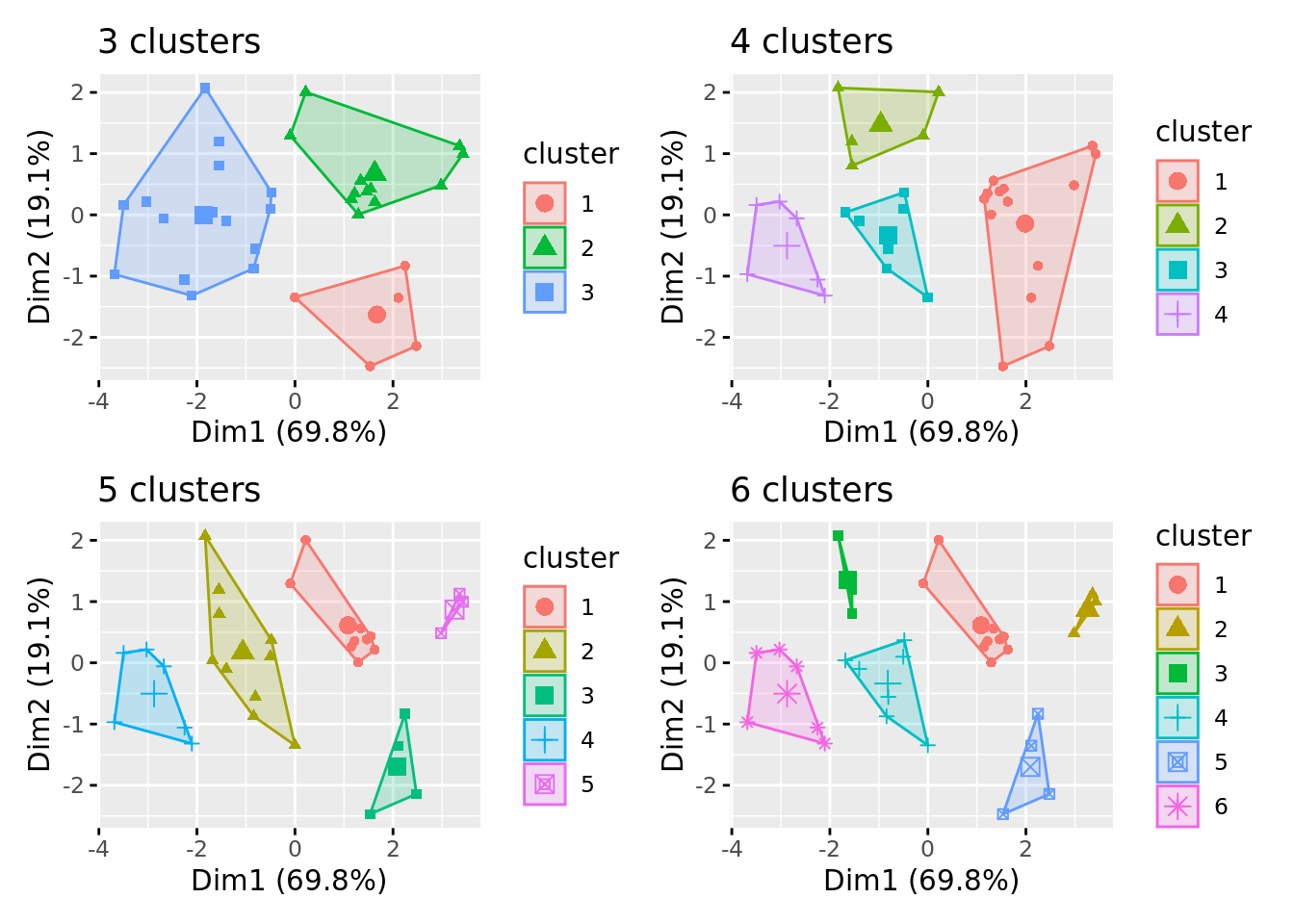

Escolhendo 5 grupos

grupo_kmeans <- data.frame(k5$cluster) |> 
  dplyr::rename (cluster = last_col())

df_final_kmeans <-  bind_cols(mtcars, grupo_kmeans)

df_final_kmeans_EDA <- df_final_kmeans |>  pivot_longer(cols = c(1,3:7))

plot_final_kmeans_EDA <- df_final_kmeans_EDA |> 
  ggplot(aes(x=cluster, y=value, color= as_factor(cluster)))+
  #geom_jitter(alpha = 0.5, size = 6, width = 0.1)+
  geom_boxplot()+
  facet_grid(scales = "free_x", cols = vars(name))

plot_final_kmeans_EDA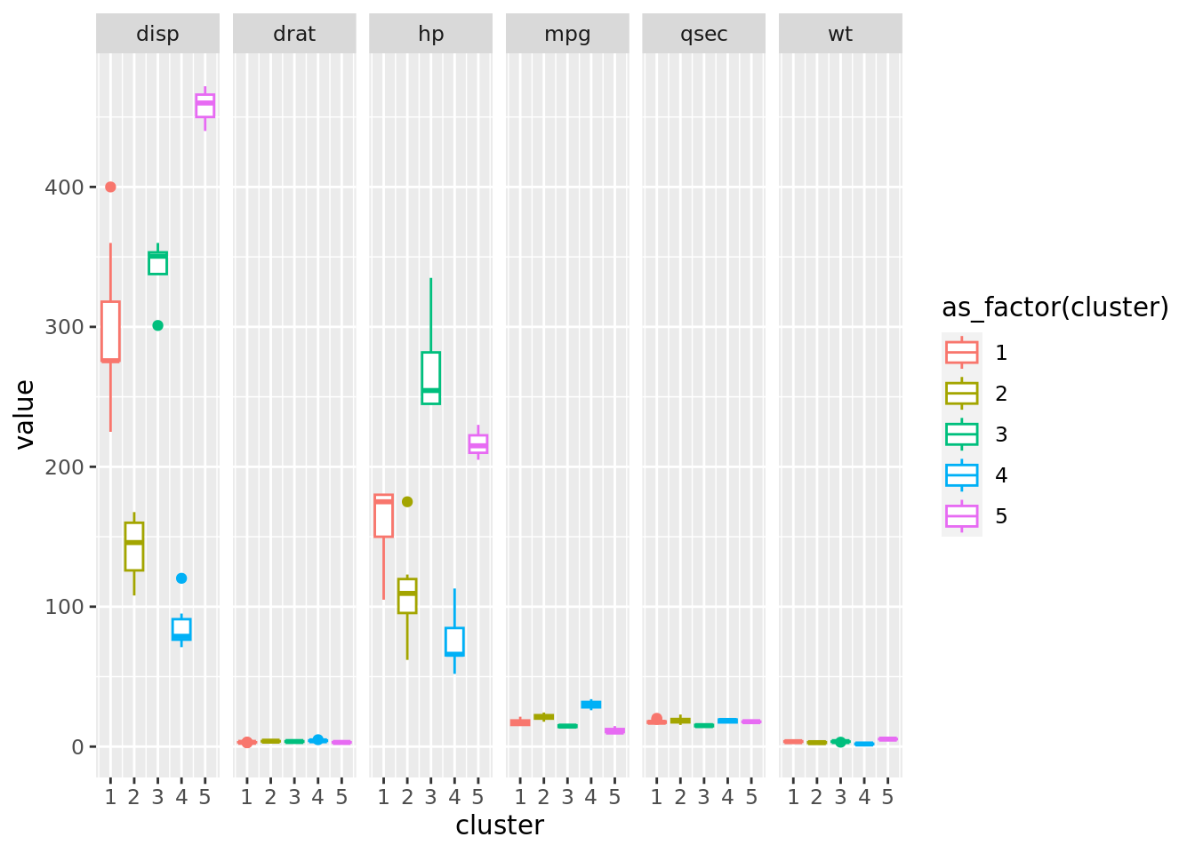

Visualizando os dados com os respetivos clsuters k-means

df_final_kmeans |> 
  group_by(cluster) |> 
  gt(rowname_col = "name") |> 
  tab_stubhead(label ="Modelo") |> 
  tab_options(row.striping.include_table_body = TRUE) |> 
  text_transform(locations = cells_row_groups(),
                 fn = function(x) {
      paste0("Cluster: ", x)
    })

mpg	cyl	disp	hp	drat	wt	qsec	vs	am	gear	carb
Cluster: 2
21.0	6	160.0	110	3.90	2.620	16.46	0	1	4	4
21.0	6	160.0	110	3.90	2.875	17.02	0	1	4	4
22.8	4	108.0	93	3.85	2.320	18.61	1	1	4	1
24.4	4	146.7	62	3.69	3.190	20.00	1	0	4	2
22.8	4	140.8	95	3.92	3.150	22.90	1	0	4	2
19.2	6	167.6	123	3.92	3.440	18.30	1	0	4	4
17.8	6	167.6	123	3.92	3.440	18.90	1	0	4	4
21.5	4	120.1	97	3.70	2.465	20.01	1	0	3	1
19.7	6	145.0	175	3.62	2.770	15.50	0	1	5	6
21.4	4	121.0	109	4.11	2.780	18.60	1	1	4	2
Cluster: 1
21.4	6	258.0	110	3.08	3.215	19.44	1	0	3	1
18.7	8	360.0	175	3.15	3.440	17.02	0	0	3	2
18.1	6	225.0	105	2.76	3.460	20.22	1	0	3	1
16.4	8	275.8	180	3.07	4.070	17.40	0	0	3	3
17.3	8	275.8	180	3.07	3.730	17.60	0	0	3	3
15.2	8	275.8	180	3.07	3.780	18.00	0	0	3	3
15.5	8	318.0	150	2.76	3.520	16.87	0	0	3	2
15.2	8	304.0	150	3.15	3.435	17.30	0	0	3	2
19.2	8	400.0	175	3.08	3.845	17.05	0	0	3	2
Cluster: 3
14.3	8	360.0	245	3.21	3.570	15.84	0	0	3	4
13.3	8	350.0	245	3.73	3.840	15.41	0	0	3	4
15.8	8	351.0	264	4.22	3.170	14.50	0	1	5	4
15.0	8	301.0	335	3.54	3.570	14.60	0	1	5	8
Cluster: 5
10.4	8	472.0	205	2.93	5.250	17.98	0	0	3	4
10.4	8	460.0	215	3.00	5.424	17.82	0	0	3	4
14.7	8	440.0	230	3.23	5.345	17.42	0	0	3	4
Cluster: 4
32.4	4	78.7	66	4.08	2.200	19.47	1	1	4	1
30.4	4	75.7	52	4.93	1.615	18.52	1	1	4	2
33.9	4	71.1	65	4.22	1.835	19.90	1	1	4	1
27.3	4	79.0	66	4.08	1.935	18.90	1	1	4	1
26.0	4	120.3	91	4.43	2.140	16.70	0	1	5	2
30.4	4	95.1	113	3.77	1.513	16.90	1	1	5	2

DBSCAN

dbscan <- fpc::dbscan(df, eps = .78, MinPts = 3)

grupo_dbscan <- data.frame(dbscan$cluster) |> 
  dplyr::rename (cluster = last_col())

df_final_dbscan <-  bind_cols(mtcars, grupo_dbscan)

df_final_dbscan_EDA <- df_final_dbscan |>  pivot_longer(cols = c(1,3:7))

plot_final_dbscan_EDA <- df_final_dbscan_EDA |> 
  ggplot(aes(x=cluster, y=value, color= as_factor(cluster)))+
  #geom_jitter(alpha = 0.5, size = 6, width = 0.1)+
  geom_boxplot()+
  facet_grid(scales = "free_x", cols = vars(name))

plot_final_dbscan_EDA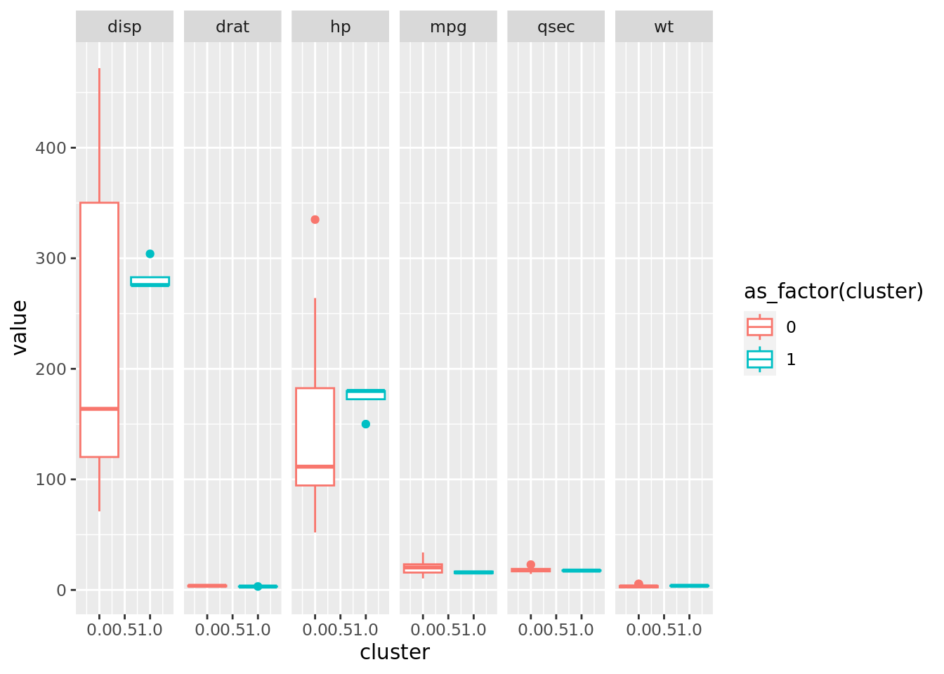

#Outros plots:
plot(dbscan, df)